1. Introduction
Large organizations generate huge amounts of internal data and
also consume data from third-party providers. These providers often
extract information from unstructured sources and invest considerable
effort in delivering it in structured form. To use this external data
effectively, it must be integrated with the company's internal
data. Such integration supports many important applications, including
a 360-degree view of the customer, fraud detection, risk assessment,
and loan approval. In this chapter, we focus on building a knowledge
graph by integrating data from structured sources. The next chapter
addresses techniques for extracting structured data from unstructured
inputs.
When integrating data from multiple sources into a knowledge graph,
we can either design a schema upfront --- as discussed in the previous
chapter --- or begin without a predefined schema and load external
data directly as triples. In practice, the initial schema is usually
guided by the specific business use case being addressed. When such a
schema exists, we must determine how the data elements in a new source
should be aligned with it. This task is known as schema
mapping.
In addition to aligning the structures of the two sources, we must
also determine whether entities in the new data correspond to entities
already represented in the knowledge graph. Inferring whether two
entity descriptions refer to the same real-world entity is known as
the record linkage problem. Record linkage arises both when
onboarding a new data source and when keeping the knowledge graph up
to date as third-party providers deliver ongoing data feeds.
In this chapter, we examine current approaches for addressing both
the schema mapping and record linkage problems. We outline
state-of-the-art algorithms and evaluate their effectiveness in
tackling contemporary industry challenges.
2. Schema Mapping
Schema mapping assumes the existence of a schema which will be used
for storing new data coming from another source. Schema mapping then
defines which relations and attributes in the input database
corresponds to which properties and relations in the knowledge
graph. There exist techniques for bootstrapping schema mappings. The
bootstrapped schema mappings can be post corrected through human
intervention.
We begin our discussion of schema mapping by outlining some of the
key challenges, emphasizing that the process is often manual and
labor-intensive. Next, we describe an approach for specifying mappings
between the schema of the input source and the schema of the knowledge
graph. Finally, we conclude the section by examining techniques that
can be used to bootstrap schema mapping and reduce the manual effort
involved.
2.1 Challenges in Schema Mapping
Automating schema mapping presents several key challenges:
understanding complex schemas, handling intricate mappings, and coping
with limited training data.
Relational database schemas can be large, often containing
thousands of tables and tens of thousands of attributes. Many
attribute names, such as segment1 or segment2, provide little semantic
meaning, making automatic mapping difficult.
Mappings between the input schema and the knowledge graph are
rarely simple one-to-one correspondences. They may require
calculations, the application of business rules, or special handling
of missing values, which makes fully automated mapping
challenging.
Finally, many automated approaches rely on machine learning, which
requires substantial training data. Because schema information is
inherently smaller and less abundant than the data itself, there are
typically too few schema mappings available to train a reliable
algorithm.
Commercial relational database schemas can be huge consisting of
thousands of relations and tens of thousands of attributes. Sometimes,
the relation and attribute names do not have semantics (e.g.,
segment1, segment2) which do not lend themseves to any realistic
automated prediction of the mappings.
2.2 Specifying Schema Mapping
In this section, we explore one approach for specifying mappings
between input data sources and a target knowledge graph schema. To
illustrate the process, we use an example from the domain of
cookware. Imagine multiple vendors providing product information that
an e-commerce site wants to aggregate and present to its customers. We
will examine two example sources and then introduce the schema of the
knowledge graph, to which we will define the mappings.
Below is some sample data from the first data source, stored in a
relational table ,called cookware. The table contains four
attributes: name, type, material,
and price.
| cookware |
|---|
| name | type | material | price |
|---|
| c01 | skillet | cast iron | 50 |
| c02 | saucepan | steel | 40 |
| c03 | skillet | steel | 30 |
| c04 | saucepan | aluminium | 20 |
|
The second database, shown below, lists the products of a
manufacturer. In this case, the data is spread across multiple
tables, each representing a different product attribute.
The kind table specifies the type of each product.
The base table specifies whether each product is made from a
corrosible metal (aluminum or stainless), a noncorrosible metal (iron
or steel), or something other than metal (glass or ceramic).
The coated table lists products that have nonstick coatings.
The price table gives the selling price. There is no
material information. The company has chosen not to provide
information about the metal used in each product. The coated
table has only positive values; products without nonstick coatings are
left unmentioned.
| kind |
|---|
| id | value |
|---|
| m01 | skillet |
| m02 | skillet |
| m03 | saucepan |
| m04 | saucepan |
|
|
| base |
|---|
| id | value |
|---|
| m01 | corrosible |
| m02 | noncorrosible |
| m03 | noncorrosible |
| m04 | nonmetallic |
|
|
| coated |
|---|
| id | value |
|---|
| m01 | yes |
| m02 | yes |
|
|
| price |
|---|
| id | value |
|---|
| m01 | 60 |
| m02 | 50 |
| m03 | 40 |
| m04 | 20 |
|
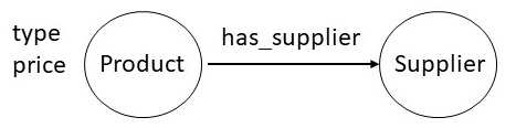
Suppose the desired schema for the knowledge graph, expressed as a
property graph, is as shown below. The graph has two different node
types: one for products, and the other for suppliers. These nodes
are connected by a relationship called has_supplier. Each
product node has properties "type" and "price".
To specify the mappings, and to illustrate the process, we will
use a triple notation, making the approach applicable whether the
knowledge graph follows the RDF or property graph data model. In the
case of an RDF knowledge graph, creating IRIs is required, but this
step is orthogonal to schema mapping and is therefore omitted here.
The desired triples in the target knowledge graph are listed
below.
| knowledge graph |
|---|
| subject | predicate | object |
|---|
| c01 | type | skillet |
| c01 | price | 50 |
| c01 | has_supplier | vendor_1 |
| c02 | type | saucepan |
| c02 | price | 40 |
| c02 | has_supplier | vendor_1 |
| c03 | type | skillet |
| c03 | price | 30 |
| c03 | has_supplier | vendor_1 |
| c04 | type | saucepan |
| c04 | price | 20 |
| c04 | has_supplier | vendor_1 |
| m01 | type | skillet |
| m01 | price | 60 |
| m01 | has_supplier | vendor_2 |
| m02 | type | skillet |
| m02 | price | 50 |
| m02 | has_supplier | vendor_2 |
| m03 | type | saucepan |
| m03 | price | 40 |
| m03 | has_supplier | vendor_2 |
| m04 | type | saucepan |
| m04 | price | 20 |
| m04 | has_supplier | vendor_2 |
|
Any programming language can be used to express the mappings. In
this example, we use Datalog to specify the mappings. The rules shown
below are straightforward, with variables indicated by uppercase
letters. The third rule introduces the constant vendor_1 to
indicate the source of the data.
knowledge_graph(ID,type,Type) :- cookware(ID,TYPE,MATERIAL,PRICE)
knowledge_graph(ID,price,PRICE) :- cookware(ID,TYPE,MATERIAL,PRICE)
knowledge_graph(ID,has_supplier,vendor_1) :- cookware(ID,TYPE,MATERIAL,PRICE)
|
Next, we consider the rules for mapping the second source. These
rules are similar to those for the first source, except that the
information now comes from two different tables in the source
data.
knowledge_graph(ID,type,Type) :- kind(ID,TYPE)
knowledge_graph(ID,price,PRICE) :- price(ID,PRICE)
knowledge_graph(ID,has_supplier,vendor_2) :- kind(ID,TYPE)
|
In general, it may not be appropriate to reuse identifiers from the
source databases, and new identifiers may need to be created for the
knowledge graph. In some cases, the knowledge graph may already
contain objects equivalent to those in the incoming data. We will
consider this issue in the section on record linkage.
2.3 Bootstrapping Schema Mapping
As noted in Section 2.1, fully automated schema mapping faces
numerous practical difficulties. Research has focused on bootrapping
the schema mappings based on a variety of techniques, with human input
often used to validate the results. Bootstrapping techniques can be
classified into three main categories: linguistic matching,
instance-based matching, and constraint-based matching. We will
examine examples of each technique in the following sections.
Linguistic techniques can be applied to attribute names or descriptions. Common approaches include:
- Exact Name Matching: Check whether the names of
two attributes are identical. Confidence is higher if the names are
expressed as IRIs.
- Canonicalization: Process names through
techniques such as stemming before checking for equality (e.g.,
mapping CName to Customer Name).
- Synonyms and Hypernyms: Identify mappings using
synonyms (e.g., car and automobile) or hypernyms
(e.g., book and publication).
- Substrings and Phonetic Similarity: Compare
attributes based on common substrings, pronunciation, or how words
sound.
- Semantic Similarity of Descriptions: Extract
keywords from attribute descriptions and assess similarity using the
techniques above.
In instance-based matching, the actual data values are examined to
determine possible mappings. For example, if an attribute contains
date values, it can only be mapped to other attributes that also
contain dates. Many standard data types can be inferred by analyzing
the data itself.
In constraint based matching, we have to rely on the the schema to
provided information about the constraints. For example, For
example, if an attribute is defined as both unique and numeric, it
is a potential match for identification fields such as an employee
number or a social security number.
The techniques considered here are inexact, and hence, can
be only used to bootstrap the schema mapping process. Any mappings
must be verified, and validated by human experts.
3. Record Linkage
We begin our discussion by illustrating the record linkage problem
with a concrete example. We then provide an overview of a typical
approach used to address record linkage in practice.
3.1 A Sample Record Linkage Problem
Suppose we have data in the two tables shown below. The record
linkage problem involves inferring that record a1 refers to
the same real-world entity as record b1, and that record
a3 refers to the same real-world entity as the record
b2. As in schema mapping, these are inexact inferences, and
need to undergo human validation.
| Table A |
|---|
| Company | City | State |
|---|
| a1 | AB Corporation | New York | NY |
| a2 | Broadway Associates | Washington | WA |
| a3 | Prolific Consulting Inc. | California | CA |
|
|
| Table B |
|---|
| Company | City | State |
|---|
| b1 | ABC | New York | NY |
| b2 | Prolific Consulting | California | CA |
|
A large knowledge graph may contain information for over 10 million
companies, and may periodically receive new data feeds extracted from
natural language text. Such feeds can contain hundreds of thousands of
companies. Even if the knowledge graph uses standardized identifiers
for companies, the incoming data extracted from text will typically
lack such identifiers. The goal of record linkage is to relate the
companies contained in this new data feed with the corresponding
companies that already exist in the knowledge graph. Because of the
large data volumes involved, performing this task efficiently is of
paramount importance.
3.2 An Approach to Solve the Record Linkage Problem
Efficient record linkage typically consists of two
stages: blocking and matching. The blocking stage
involves a fast and coarse grained computation to select a subset of
records from the source and the target datasets that are likely to
match. This reduces the number of comparisons required in the
subsequent, more expensive matching stage. During matching, records
within each block are compared pairwise using more precise
criteria.
In the example considered above, a simple blocking strategy might
consider only records that share the same state. Under this strategy,
only records a1 and b1, and a3 and
b2 need to be compared, significantly reducing the
comparisons required.
Both the blocking and matching stages can be implemented using a
random forest trained through an active learning process. A random
forest is an ensemble of decision trees, where each tree makes a
prediction and the final decision is determined by a majority
vote. This approach is well suited to record linkage because it can
combine many weak, noisy signals -- such as partial name matches or
similar addresses -- into a robust overall decision.
Active learning further improves efficiency by focusing human
effort where it is most valuable. Instead of labeling a large number
of random training examples, the model actively identifies cases where
it is uncertain and requests human input for those examples. These
labeled examples are then used to iteratively refine the random
forest. Together, random forests and active learning provide an
effective and scalable approach to both blocking and matching.
3.3 Blocking
Blocking rules rely on standard similarity checking functions, such
as, exact match, Jaccard similarity, overlap similarity, cosine
similarity, etc. For example, to compute the overlap similarity
between "Prolific Consulting" and "Prolific Consulting Inc.", we will
first gather the tokens in each of them, and then check which tokens
are in common, giving us a similarity score of 2/3.
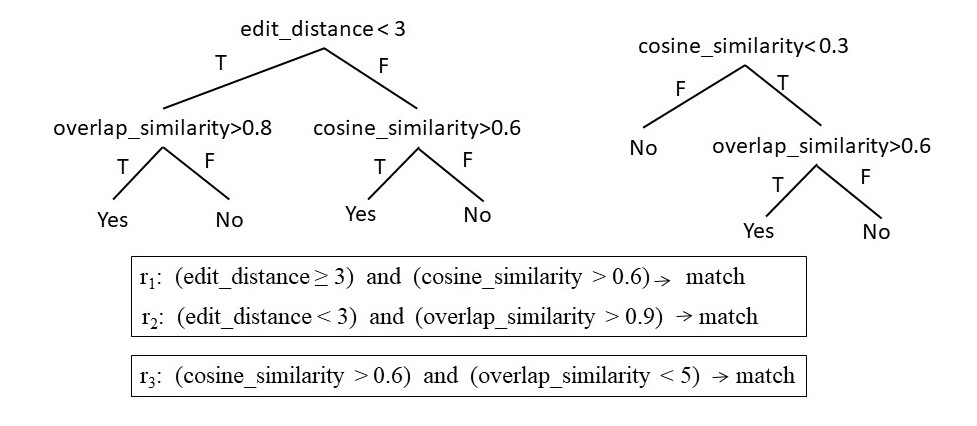
Below is a snippet of a random forest used for blocking. A random
forest can also be viewed as a collection of rule sets. The random
forest shown below consists of two sets of rules. The arguments of
each predicate are two values to be compared.
Several general principles guide the automatic selection of the
similarity functions for blocking. For numerical
attributes such as age, weight, price, etc., candidate
similarity functions include exact match, absolute difference, relative
difference, and Levenstein distance. For string valued attributes, typical
choices include edit distance, cosine similarity, Jaccard similarity,
and TF/IDF-based similarity measures.
3.4 Active Learning of Random Forests
We can learn the random forest for the blocking rules through
the following active learning process. First, we randomly select a
set of record pairs from the two datasets. By applying the
similarity functions to each pair, we generate a set of feautres
for each pair. Using these features, we train a random forest. The
resulting rules are then aplied to new record pairs, and their
performance evaluated. If the performance falls below a specified
threshold, the process is repeated by providing additional labeled
examples until an acceptable performance is obtained. We
illustrate this process using the following example.
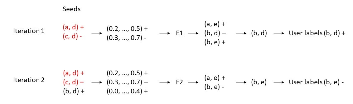
Suppose our first dataset contains three
items: a, b, and c, and our second
dataset contains two items: d and e. From these
datasets, we select two pairs, (a, d) and (c, d),
which are labeled by the user as similar and not similar,
respectively.
For each pair, we apply the
similarity functions to generate
features, which are then used to train a random forest. The learned
rules are applied to the remaining pairs not in the training set, and
the user verifies the results. If the user identifies an incorrect
prediction, such as for the pair (b, d), it is added to the
training set for the next iteration.
Repeating this process over several iterations allows the random
forest to converge to a model that can be effectively used in the
blocking step.
Once a radom forest has been learned, we present each of the learned rules to
the user. Based on the user verification, we choose the rules that will be
used in the subsequent steps.
3.5 Applying the Rules
Once the blocking rules have been learned, the next step is to
apply them to the actual data. When the dataset is very large, it is
impractical to apply the rules to all possible pairs of objects. To
address this, we use indexing.
For example, suppose one rule requires that the Jaccard index
between two strings be greater than 0.7, and we want to match the
movie Sound of Music. Since the length of this movie name is
3, we only need to consider movies whose lengths are between 3 ×
0.7 and 3 / 0.7, i.e., between 2 and 4. If the
dataset is indexed by string length, we can efficiently select only
those movies with lengths in this range and then further filter them
by applying the blocking rule.
3.6 Matching
The blocking step produces a much smaller set of record pairs that
need to be evaluated for matches. The structure of the matching
process is similar: we first define a set of features, train a random
forest, and iteratively refine it through active learning. The primary
difference between blocking and matching is that the matching step
requires greater precision and often more computation. This is because
matching is the final step in record linkage, and it is essential to
have high confidence that the two records indeed refer to the same
real-world entity.
4. Summary
In this chapter, we examined the problem of creating a knowledge
graph by integrating data from structured sources. The integrated
schema of the knowledge graph can be refined and evolved to meet
changing business requirements. Mappings between the schemas of
different sources can be bootstrapped using automated techniques, but
they still require verification by human experts. Record linkage
addresses integration at the instance level, where we must infer
whether two records refer to the same real-world entity in the absence
of unique identifiers. A common approach for record linkage is to
learn a random forest through an active learning process. For
applications that demand high accuracy, automatically computed record
linkages may also require human validation.
5. Further Reading
The schema mapping problem has attracted attention of both database
researchers [Rahm
& Bernstein 2001] and ontology
researchers [Noy
& Stuckenschmidt 2005] with each community producing its own
survey of techniques. Ontology Alignment
Evaluation Initiative (OAEI) is an international effort to evaluate
and compare ontology and schema matching techniques in a standardized
way [OAEI]. Its
primary goals are to assess the strengths and weaknesses of alignment
systems, compare performance across methods, improve evaluation
techniques, and foster communication among researchers.
The disucssion on the record linkage in this chapter is based on
the Magellan system developed at University of Wisconsin at
Madison [Doan
et. al. 2020]. Record linking is referred to by several other
names including deduplication and entity resolution. For an
appreciation of the complexities of real-world record linking, refer
to the explanation by Jeff
Jonas [Jonas
21]. Recent trends on record linking include leveraging deep
learning
architectures [Mudgal
et. al. 2020] including the recent Large Language
Models [Peeters
& Bizer 2023].
[Rahm
& Bernstein 2001] Rahm, Erhard, and Philip A. Bernstein. "A survey
of approaches to automatic schema matching." the VLDB Journal 10.4
(2001): 334-350.
[Noy
& Stuckenschmidt 2005] Noy, Natasha, and Heiner
Stuckenschmidt. "Ontology alignment: An annotated bibliography."
Schloss Dagstuhl–Leibniz-Zentrum für Informatik, 2005.
[OAEI] Ontology
Alignment Evaluation Initiative. (n.d.). Ontology Alignment Evaluation
Initiative. Retrieved December 12, 2025, from
https://oaei.ontologymatching.org/
[Doan
et. al. 2020] Doan, A., Konda, P., Paulsen, D., Chandrasekhar, K.,
Martinkus, P., Christie, M., Govind, Y., & Suganthan,
P. C. (2020). Magellan: Toward building ecosystems of entity matching
solutions. Communications of the ACM, 63(8),
83–91. https://doi.org/10.1145/3405476
[Jonas
21] Jonas, J. (2021, approx.). Entity resolution explained step by
step [Video]. YouTube. https://www.youtube.com/watch?v=VFE3kGdoXzA
[Mudgal
et. al. 2020] Mudgal, S., Li, H., Rekatsinas, T., Doan, A., Park,
Y., Krishnan, G., Deep, R., Arcaute, E., & Raghavendra,
V. (2018). Deep learning for entity matching: A design space
exploration. In Proceedings of the 2018 International Conference on
Management of Data (SIGMOD ’18)
(pp. 19–34). ACM. https://doi.org/10.1145/3183713.319692
[Peeters &
Bizer 2023] Peeters, R., & Bizer, C. (2023). Using ChatGPT for
entity matching (arXiv:2305.03423)
[Preprint]. arXiv. https://doi.org/10.48550/arXiv.2305.03423
Exercises
Exercise 4.1.Two
popular methods to calculate similarity between two strings are
edit distance (also known as Levenshtein distance) and the Jaccard measure.
We can define the
Levenshtein distance between two strings a, b (of length |a| and |b|
respectively), given by lev(a,b) as follows:
- lev(a,b) = a if |b| = 0
- lev(a,b) = b if |a| = 0
- lev(tail(a),tail(b)), if a[0] = b[0]
- 1 + min{lev(tail(a),b), lev(a,tail(b)), lev(tail(a),tail(b))} otherwise.
where the tail of some string x is a string of all but the first
character of x, and x[n] is the nth character of the string x,
starting with character 0.
We can define the Jaccard measure between two strings a, b
as the size of the intersection divided by the size of the
union between the two.
J(a,b) = |a ∩ b| / |a ∪ b|
|
(a) |
Given the strings "JP Morgan Chase" and "JPMC Corporation", what is the edit distance between the two? |
|
(b) |
Given the strings "JP Morgan Chase" and "JPMC Corporation", what is the Jaccard measure between the two? |
|
(c) |
Given three strings: x = Apple Corporation, CA, y = IBM Corporation, CA, and z =
Apple Corp, which of these strings would be equated by the edit distance methods? |
|
(d) |
Given three strings: x = Apple Corporation, CA, y = IBM Corporation, CA, and z =
Apple Corp, which of these strings will be equated by the Jaccard measure? |
|
(e) |
Given three strings: x = Apple Corporation, CA, y = IBM Corporation, CA, and z =
Apple Corp, what intuition you would use to ensure that x is equated to z? |
Exercise
4.2. A commonly used approach to account for the importance
of words is a measure known as TF/IDF. Term frequency (TF) denotes
the number of times a term occurs in a document. Inverse Document
Frequency (IDF) denotes the number of documents containing a term.
The TF/IDF score is calculated by taking the product of TF and
IDF. Use your intuition to answer whether the following is true
or false.
|
(a) |
Higher the TF/IDF score of a word, the rarer it is. |
|
(b) |
In a general news corpus, TF/IDF for the word Apple is likely to be higher than the TF/IDF for the word Corporation |
|
(c) |
Common words such as stop words will have a high TF/IDF. |
|
(d) |
If a document contains words with high TF/IDF, it is likely to be ranked higher by the search engines. |
|
(e) |
The concept of TF/IDF is not limited to words, and can also be applied to sequence of characters, for example, bigrams. |
Exercise
4.3. To check if two names might refer to the same
real-world organization, one strategy is to check the similarity
between two documents that describe them. Cosine similarity is a
measure of similarity between two vectors, and is defined as the
cosine of the angle between them. Highly similar documents will
have a cosine score closer to 1. Which of the following might be
a viable approach to convert a document into a vector for calculating
cosine similarity?
|
(a) |
Word embeddings of the words used in a document. |
|
(b) |
TF/IDF scores of the words used in a document. |
|
(c) |
TF/IDF of bigrams used in a document. |
|
(d) |
None of the above. |
|
(e) |
Any of (a), (b) or (c). |
Exercise
4.4. Which of the following is true about schema mappings?
|
(a) |
Schema mapping is largely an automated process. |
|
(b) |
It is usually straightforward to learn simple schema mappings. |
|
(c) |
Complete schema documentation is almost never available. |
|
(d) |
Examining the actual data in the two sources can provide important clues for schema mapping. |
|
(e) |
Database constraints play no role in schema mapping. |
Exercise
4.5. Which of the following is true about record linkage?
|
(a) |
Blocking can be an unnecessary and expensive step in the record linkage pipeline. |
|
(b) |
A random forest is a set of set of rules. |
|
(c) |
Blocking rules must always be authored manually. |
|
(d) |
Active learning of blocking rules minimizes the training data we must provide. |
|
(e) |
Matching rules are as expensive to apply as the blocking rules. |
Exercise 4.6. Implement a schema mapper for
the conference
domain of the Ontology Alignment Evaluation Initiative. The
domain consists of 16 different schemas describing conferences.
Exercise 4.7. Create a knowledge graph of companies by
linking the records across Wikidata and the SEC data considered as
part the problem 3.7. To connect the two data sets, you can either
implement your own record linker, or use any available open-source
tools. Report on the quality of the resulting data set in terms of the
precision and recall of identifying the correct links across the SEC
company data and the Wikidata company information.
|
 CS520
CS520